11  Hypoplastic MDS

Biology, Diagnosis, and Clinical Management

Author

Clinical Research Analysis

Published

August 19, 2026

12 Introduction

Hypoplastic myelodysplastic syndrome (h-MDS) represents a distinct clinical entity comprising 10-15% of all MDS cases. This subtype occupies a unique pathobiological position between aplastic anemia (AA) and normo/hypercellular MDS, with important implications for diagnosis, prognosis, and therapeutic approach.

The 2022 WHO Classification formally recognizes MDS-hypoplastic (MDS-h) as a morphologically-defined entity, validating decades of clinical observations that these patients respond differently to treatment and have distinct outcomes compared to typical MDS.

12.1 Key Clinical Features

Show code
key_features <- tribble(
  ~Feature, ~`h-MDS`, ~`n-MDS`, ~`AA`,
  "Bone marrow cellularity", "<25-30%", ">30%", "<25%",
  "Dysplasia", "Present (≥10%)", "Present (≥10%)", "Absent/minimal",
  "Blasts", "<5%", "Variable", "0%",
  "PNH clones", "24-43%", "~2%", ">50%",
  "Somatic mutations", "35-38%", "62-65%", "Variable",
  "IST response rate", "46-49%", "21-24%", "60-70%"
)

key_features %>%
  gt() %>%
  tab_header(
    title = "Comparison of Hypoplastic MDS with Related Disorders",
    subtitle = "Key diagnostic and clinical features"
  ) %>%
  tab_spanner(
    label = "Disease Entity",
    columns = c(`h-MDS`, `n-MDS`, `AA`)
  ) %>%
  cols_align(align = "center", columns = -Feature) %>%
  tab_style(
    style = cell_fill(color = "#E8F4F8"),
    locations = cells_body(columns = `h-MDS`)
  ) %>%
  tab_footnote(
    footnote = "IST = Immunosuppressive therapy; PNH = Paroxysmal nocturnal hemoglobinuria",
    locations = cells_column_labels(columns = Feature)
  )
Comparison of Hypoplastic MDS with Related Disorders
Key diagnostic and clinical features
Feature1
Disease Entity
h-MDS n-MDS AA
Bone marrow cellularity <25-30% >30% <25%
Dysplasia Present (≥10%) Present (≥10%) Absent/minimal
Blasts <5% Variable 0%
PNH clones 24-43% ~2% >50%
Somatic mutations 35-38% 62-65% Variable
IST response rate 46-49% 21-24% 60-70%
1 IST = Immunosuppressive therapy; PNH = Paroxysmal nocturnal hemoglobinuria
Figure 12.1: Key distinguishing features of hypoplastic MDS

13 Epidemiology and Classification

13.1 WHO 2022 Classification Criteria

The WHO 2022 5th edition establishes specific diagnostic criteria for MDS-hypoplastic:

Show code
who_criteria <- tribble(
  ~Criterion, ~Specification,
  "Bone marrow cellularity", "<30% if age <70 years; <20% if age ≥70 years",
  "Dysplasia", "≥10% in at least one hematopoietic lineage",
  "Blast percentage", "<5% in bone marrow",
  "Cytopenias", "At least one cytopenia meeting MDS thresholds",
  "Exclusions", "Somatic PIGA mutations must be absent",
  "Additional exclusions", "Inherited bone marrow failure syndromes must be excluded"
)

who_criteria %>%
  gt() %>%
  tab_header(
    title = "WHO 2022 Diagnostic Criteria for MDS-Hypoplastic"
  ) %>%
  cols_width(
    Criterion ~ px(200),
    Specification ~ px(400)
  ) %>%
  tab_style(
    style = cell_text(weight = "bold"),
    locations = cells_body(columns = Criterion)
  )
Table 13.1
WHO 2022 Diagnostic Criteria for MDS-Hypoplastic
Criterion Specification
Bone marrow cellularity <30% if age <70 years; <20% if age ≥70 years
Dysplasia ≥10% in at least one hematopoietic lineage
Blast percentage <5% in bone marrow
Cytopenias At least one cytopenia meeting MDS thresholds
Exclusions Somatic PIGA mutations must be absent
Additional exclusions Inherited bone marrow failure syndromes must be excluded

13.2 Incidence by Age

Show code
# Simulated age distribution based on published data
set.seed(42)
age_data <- tibble(
  age_group = factor(c("<40", "40-49", "50-59", "60-69", "70-79", "≥80"),
                     levels = c("<40", "40-49", "50-59", "60-69", "70-79", "≥80")),
  h_mds_pct = c(5, 8, 15, 28, 30, 14),
  n_mds_pct = c(2, 5, 12, 30, 35, 16)
)

age_data_long <- age_data %>%
  pivot_longer(cols = c(h_mds_pct, n_mds_pct),
               names_to = "type",
               values_to = "percentage") %>%
  mutate(type = case_when(
    type == "h_mds_pct" ~ "Hypoplastic MDS",
    type == "n_mds_pct" ~ "Normo/Hypercellular MDS"
  ))

ggplot(age_data_long, aes(x = age_group, y = percentage, fill = type)) +
  geom_col(position = "dodge", alpha = 0.85) +
  scale_fill_manual(values = c("Hypoplastic MDS" = "#2E86AB", 
                               "Normo/Hypercellular MDS" = "#A23B72")) +
  labs(
    x = "Age Group (years)",
    y = "Percentage of Patients (%)",
    fill = "MDS Subtype",
    title = "Age Distribution in MDS Subtypes",
    subtitle = "Hypoplastic MDS shows slightly younger age at presentation"
  ) +
  scale_y_continuous(labels = scales::percent_format(scale = 1)) +
  theme(legend.position = "top")
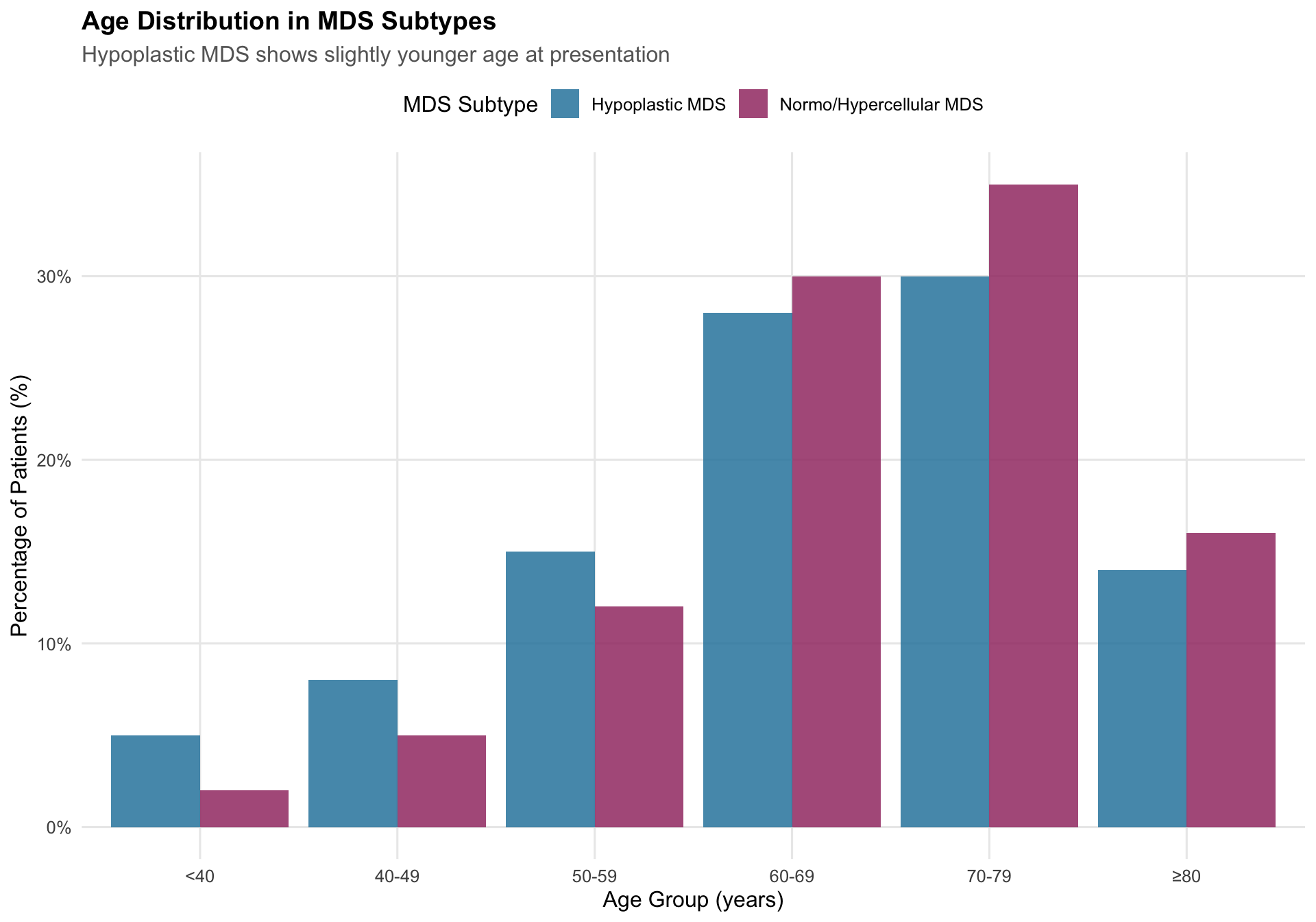
Figure 13.1: Age distribution of hypoplastic MDS patients

14 Biology and Pathogenesis

14.1 Dual Pathogenic Mechanisms

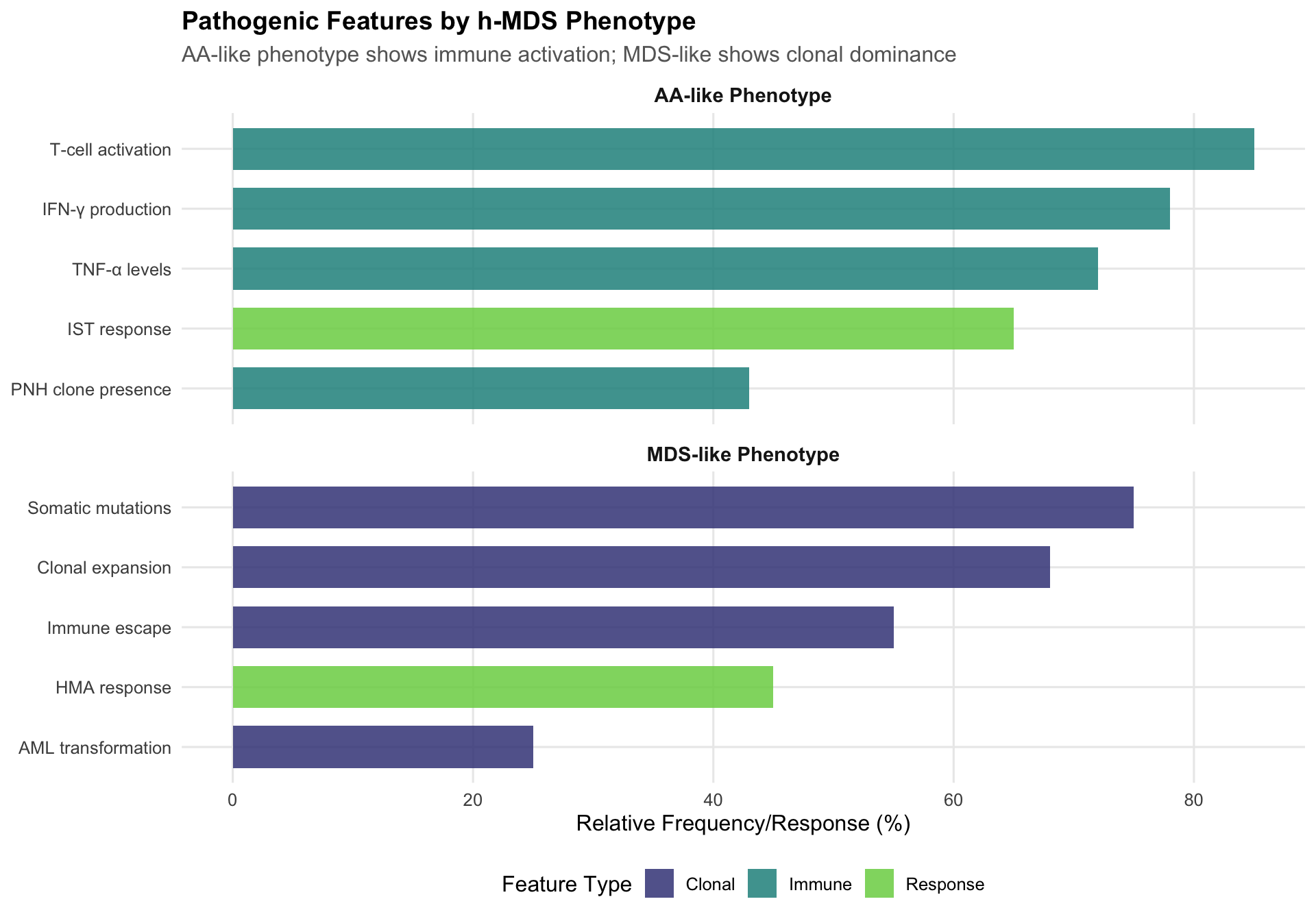
Hypoplastic MDS exhibits two distinct phenotypes with different underlying biology:

Show code
pathogenesis_data <- tribble(
  ~Mechanism, ~Feature, ~Value, ~Category,
  "AA-like Phenotype", "T-cell activation", 85, "Immune",
  "AA-like Phenotype", "IFN-γ production", 78, "Immune",
  "AA-like Phenotype", "TNF-α levels", 72, "Immune",
  "AA-like Phenotype", "PNH clone presence", 43, "Immune",
  "AA-like Phenotype", "IST response", 65, "Response",
  "MDS-like Phenotype", "Somatic mutations", 75, "Clonal",
  "MDS-like Phenotype", "Clonal expansion", 68, "Clonal",
  "MDS-like Phenotype", "Immune escape", 55, "Clonal",
  "MDS-like Phenotype", "AML transformation", 25, "Clonal",
  "MDS-like Phenotype", "HMA response", 45, "Response"
)

ggplot(pathogenesis_data, aes(x = reorder(Feature, Value), y = Value, fill = Category)) +
  geom_col(alpha = 0.85, width = 0.7) +
  coord_flip() +
  facet_wrap(~Mechanism, scales = "free_y", ncol = 1) +
  scale_fill_viridis_d(option = "D", begin = 0.2, end = 0.8) +
  labs(
    x = NULL,
    y = "Relative Frequency/Response (%)",
    fill = "Feature Type",
    title = "Pathogenic Features by h-MDS Phenotype",
    subtitle = "AA-like phenotype shows immune activation; MDS-like shows clonal dominance"
  ) +
  theme(strip.text = element_text(face = "bold", size = 11))
Figure 14.1: Dual pathogenic mechanisms in hypoplastic MDS

14.2 Immune Dysregulation

Show code
immune_markers <- tribble(
  ~Marker, ~`h-MDS`, ~`n-MDS`, ~`AA`, ~`Clinical Significance`,
  "CD8+ T cells", "↑↑", "↑", "↑↑↑", "Cytotoxic effector expansion",
  "Treg cells", "↓", "↓↓", "↓↓", "Loss of immune regulation",
  "IFN-γ expressing CD4+", "↑↑", "↑", "↑↑↑", "Th1 polarization",
  "IL-10 levels", "↓", "↑", "↓↓", "Reduced anti-inflammatory",
  "TNF-α monocytes", "↑↑", "↑", "↑↑", "Inflammatory drive",
  "PNH clone size", "0.4%*", "Rare", "2-5%*", "Immune escape marker"
)

immune_markers %>%
  gt() %>%
  tab_header(
    title = "Immune Marker Profile in Bone Marrow Failure Syndromes"
  ) %>%
  cols_align(align = "center", columns = -c(Marker, `Clinical Significance`)) %>%
  tab_style(
    style = cell_fill(color = "#FFF3E0"),
    locations = cells_body(
      columns = c(`h-MDS`, `n-MDS`, `AA`),
      rows = everything()
    )
  ) %>%
  tab_footnote(
    footnote = "*Median clone size in granulocytes",
    locations = cells_body(columns = `h-MDS`, rows = 6)
  )
Table 14.1
Immune Marker Profile in Bone Marrow Failure Syndromes
Marker h-MDS n-MDS AA Clinical Significance
CD8+ T cells ↑↑ ↑ ↑↑↑ Cytotoxic effector expansion
Treg cells ↓ ↓↓ ↓↓ Loss of immune regulation
IFN-γ expressing CD4+ ↑↑ ↑ ↑↑↑ Th1 polarization
IL-10 levels ↓ ↑ ↓↓ Reduced anti-inflammatory
TNF-α monocytes ↑↑ ↑ ↑↑ Inflammatory drive
PNH clone size 0.4%*1 Rare 2-5%* Immune escape marker
1 *Median clone size in granulocytes

15 Molecular Landscape

15.1 Mutation Frequencies

Show code
mutation_data <- tribble(
  ~Gene, ~h_MDS, ~n_MDS, ~AA,
  "SF3B1", 11, 29, 2,
  "SRSF2", 5, 14, 1,
  "U2AF1", 4, 11, 1,
  "TET2", 10, 21, 5,
  "DNMT3A", 8, 18, 8,
  "ASXL1", 5, 18, 7,
  "TP53", 3, 11, 2,
  "RUNX1", 3, 9, 1,
  "EZH2", 1, 5, 0,
  "BCOR", 6, 4, 15,
  "PIGA", 3, 0.5, 25
)

mutation_long <- mutation_data %>%
  pivot_longer(cols = c(h_MDS, n_MDS, AA),
               names_to = "Disease",
               values_to = "Frequency") %>%
  mutate(Disease = case_when(
    Disease == "h_MDS" ~ "h-MDS",
    Disease == "n_MDS" ~ "n-MDS",
    Disease == "AA" ~ "Aplastic Anemia"
  ),
  Disease = factor(Disease, levels = c("h-MDS", "n-MDS", "Aplastic Anemia")))

ggplot(mutation_long, aes(x = reorder(Gene, -Frequency), y = Frequency, fill = Disease)) +
  geom_col(position = position_dodge(width = 0.8), width = 0.7, alpha = 0.85) +
  scale_fill_manual(values = c("h-MDS" = "#2E86AB", 
                               "n-MDS" = "#A23B72",
                               "Aplastic Anemia" = "#F18F01")) +
  labs(
    x = "Gene",
    y = "Mutation Frequency (%)",
    fill = "Disease",
    title = "Somatic Mutation Frequencies by Disease Entity",
    subtitle = "h-MDS shows intermediate mutation burden between AA and n-MDS"
  ) +
  theme(
    axis.text.x = element_text(angle = 45, hjust = 1, face = "italic"),
    legend.position = "top"
  ) +
  geom_hline(yintercept = 0, color = "gray30")
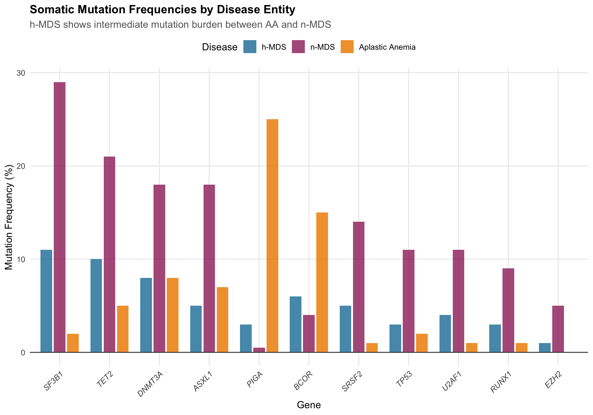
Figure 15.1: Somatic mutation frequencies across MDS subtypes and aplastic anemia

15.2 Mutation Summary Statistics

Show code
mutation_stats <- tribble(
  ~Parameter, ~`h-MDS`, ~`n-MDS`, ~`AA`, ~`p-value`,
  "Patients with ≥1 mutation", "35-38%", "62-65%", "20-30%", "<0.001",
  "Median mutations per patient", "0.5", "1.8", "0.3", "<0.001",
  "Median VAF", "15%", "25%", "8%", "<0.01",
  "Splicing factor mutations", "15%", "35%", "3%", "<0.001",
  "DTA mutations*", "18%", "42%", "15%", "<0.001",
  "TP53 mutations", "3%", "11%", "2%", "0.02"
)

mutation_stats %>%
  gt() %>%
  tab_header(
    title = "Molecular Characteristics by Disease Entity",
    subtitle = "h-MDS demonstrates intermediate clonal burden"
  ) %>%
  cols_align(align = "center", columns = -Parameter) %>%
  tab_style(
    style = cell_text(weight = "bold"),
    locations = cells_body(columns = `p-value`, rows = `p-value` == "<0.001")
  ) %>%
  tab_footnote(
    footnote = "*DTA = DNMT3A, TET2, ASXL1 mutations",
    locations = cells_body(columns = Parameter, rows = 5)
  ) %>%
  tab_source_note(
    source_note = "VAF = Variant allele frequency"
  )
Table 15.1
Molecular Characteristics by Disease Entity
h-MDS demonstrates intermediate clonal burden
Parameter h-MDS n-MDS AA p-value
Patients with ≥1 mutation 35-38% 62-65% 20-30% <0.001
Median mutations per patient 0.5 1.8 0.3 <0.001
Median VAF 15% 25% 8% <0.01
Splicing factor mutations 15% 35% 3% <0.001
DTA mutations*1 18% 42% 15% <0.001
TP53 mutations 3% 11% 2% 0.02
1 *DTA = DNMT3A, TET2, ASXL1 mutations
VAF = Variant allele frequency

15.3 Cytogenetic Abnormalities

Show code
cyto_data <- tribble(
  ~Abnormality, ~h_MDS, ~n_MDS,
  "Normal karyotype", 65, 45,
  "Trisomy 8", 12, 8,
  "del(20q)", 8, 6,
  "del(5q)", 3, 12,
  "del(7q)/-7", 4, 15,
  "Complex (≥3)", 3, 12,
  "Other", 5, 12
)

cyto_long <- cyto_data %>%
  pivot_longer(cols = c(h_MDS, n_MDS),
               names_to = "Type",
               values_to = "Percentage") %>%
  mutate(Type = ifelse(Type == "h_MDS", "Hypoplastic MDS", "Normo/Hypercellular MDS"))

ggplot(cyto_long, aes(x = Abnormality, y = Percentage, fill = Type)) +
  geom_col(position = "dodge", alpha = 0.85) +
  scale_fill_manual(values = c("Hypoplastic MDS" = "#2E86AB",
                               "Normo/Hypercellular MDS" = "#A23B72")) +
  coord_flip() +
  labs(
    x = NULL,
    y = "Frequency (%)",
    fill = "MDS Subtype",
    title = "Cytogenetic Abnormalities in MDS Subtypes",
    subtitle = "h-MDS shows higher rate of normal karyotype and lower high-risk abnormalities"
  ) +
  theme(legend.position = "top")
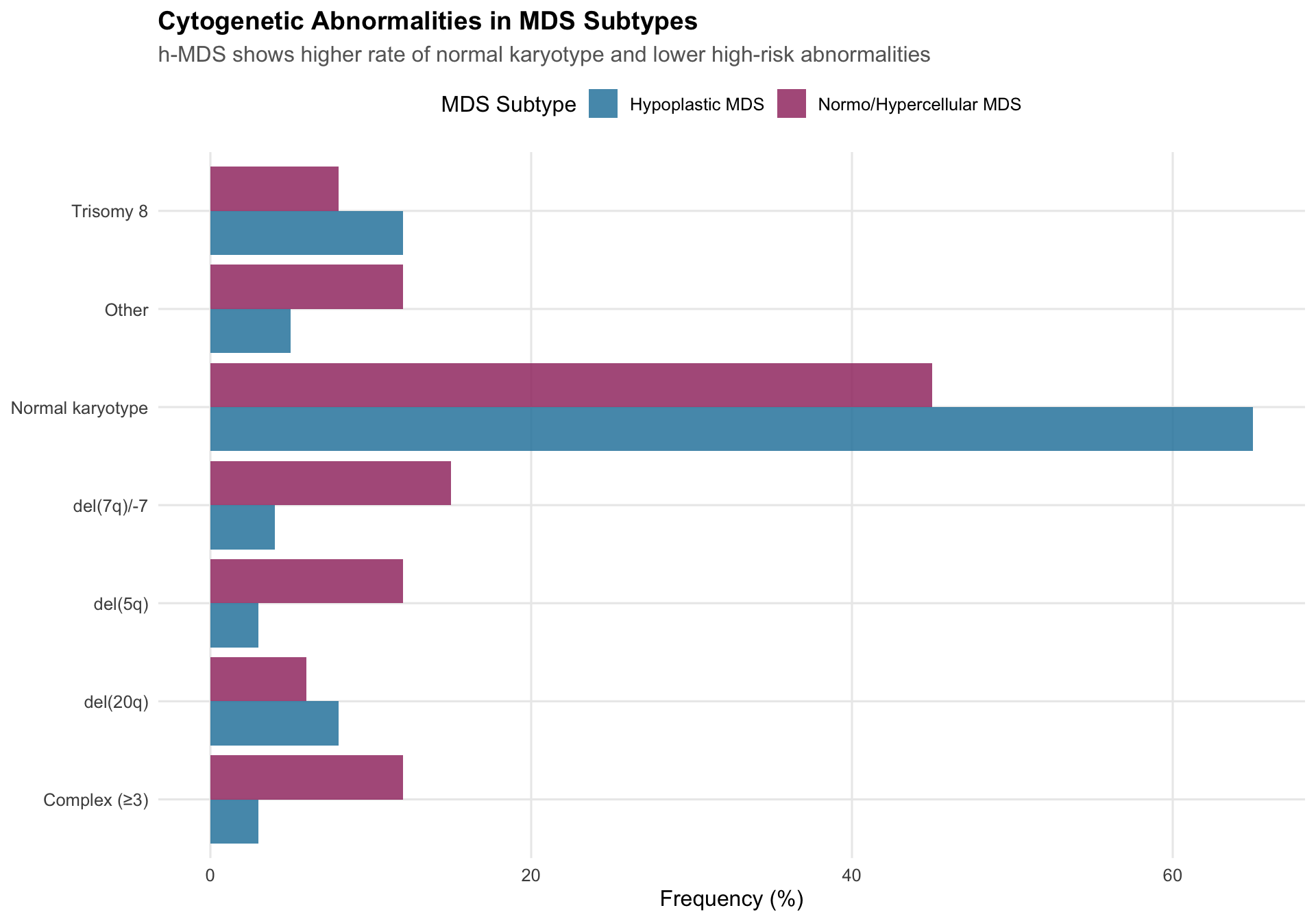
Figure 15.2: Cytogenetic abnormality frequencies in hypoplastic vs normo/hypercellular MDS

16 Differential Diagnosis

16.1 Distinguishing h-MDS from Aplastic Anemia

Show code
diff_dx <- tribble(
  ~Feature, ~`Favors h-MDS`, ~`Favors AA`, ~`Diagnostic Weight`,
  "Blast percentage", "≥2%", "0%", "+++",
  "Multilineage dysplasia", "Present", "Absent", "+++",
  "Megakaryocyte dysplasia", "Present", "Absent/rare", "++",
  "Ring sideroblasts", "Present", "Absent", "+++",
  "Cytogenetic abnormalities", "50%", "10-15%", "++",
  "MDS-type mutations", "SF3B1, SRSF2, U2AF1", "PIGA, BCOR", "++",
  "CD34+ clusters (ALIP)", "Present", "Absent", "++",
  "PNH clone size", "<1%", ">1%", "+",
  "HLA-DR15 positivity", "Variable", "Common", "+"
)

diff_dx %>%
  gt() %>%
  tab_header(
    title = "Differential Diagnosis: h-MDS vs Aplastic Anemia",
    subtitle = "Features favoring each diagnosis"
  ) %>%
  cols_align(align = "center", columns = `Diagnostic Weight`) %>%
  tab_style(
    style = cell_fill(color = "#E3F2FD"),
    locations = cells_body(columns = `Favors h-MDS`)
  ) %>%
  tab_style(
    style = cell_fill(color = "#FFF8E1"),
    locations = cells_body(columns = `Favors AA`)
  ) %>%
  tab_footnote(
    footnote = "+++ = Strong discriminator; ++ = Moderate; + = Weak",
    locations = cells_column_labels(columns = `Diagnostic Weight`)
  )
Table 16.1
Differential Diagnosis: h-MDS vs Aplastic Anemia
Features favoring each diagnosis
Feature Favors h-MDS Favors AA Diagnostic Weight1
Blast percentage ≥2% 0% +++
Multilineage dysplasia Present Absent +++
Megakaryocyte dysplasia Present Absent/rare ++
Ring sideroblasts Present Absent +++
Cytogenetic abnormalities 50% 10-15% ++
MDS-type mutations SF3B1, SRSF2, U2AF1 PIGA, BCOR ++
CD34+ clusters (ALIP) Present Absent ++
PNH clone size <1% >1% +
HLA-DR15 positivity Variable Common +
1 +++ = Strong discriminator; ++ = Moderate; + = Weak

16.2 Histologic-Genetic Score (hg-score)

Show code
hg_score <- tribble(
  ~Component, ~Finding, ~Points,
  "Bone marrow blasts", "≥5%", "2",
  "Bone marrow blasts", "2-4%", "1",
  "Fibrosis", "Grade 2-3", "1",
  "Dysmegakaryopoiesis", "Present", "1",
  "Ring sideroblasts", "≥15%", "1",
  "Severe dysgranulopoiesis", "Present", "1",
  "Cytogenetic abnormalities", "MDS-related", "2",
  "Somatic mutations", "MDS-type", "1"
)

hg_score %>%
  gt() %>%
  tab_header(
    title = "Histologic-Genetic (hg) Score Components",
    subtitle = "Score ≥2 = 98% specificity for h-MDS over AA"
  ) %>%
  cols_align(align = "center", columns = Points) %>%
  tab_row_group(
    label = "Histologic Features",
    rows = 1:6
  ) %>%
  tab_row_group(
    label = "Genetic Features",
    rows = 7:8
  ) %>%
  tab_style(
    style = cell_text(weight = "bold"),
    locations = cells_body(columns = Points)
  )
Table 16.2
Histologic-Genetic (hg) Score Components
Score ≥2 = 98% specificity for h-MDS over AA
Component Finding Points
Genetic Features
Cytogenetic abnormalities MDS-related 2
Somatic mutations MDS-type 1
Histologic Features
Bone marrow blasts ≥5% 2
Bone marrow blasts 2-4% 1
Fibrosis Grade 2-3 1
Dysmegakaryopoiesis Present 1
Ring sideroblasts ≥15% 1
Severe dysgranulopoiesis Present 1

17 Treatment Algorithm

17.1 Treatment Decision Framework

Show code
# Create treatment algorithm visualization
treatment_flow <- tribble(
  ~Step, ~Category, ~Option, ~Value, ~Label,
  1, "Assessment", "Confirm h-MDS diagnosis", 100, "WHO 2022 criteria",
  2, "Risk", "Low/Int-1 IPSS-R", 70, "Consider IST",
  2, "Risk", "Int-2/High IPSS-R", 30, "Consider HMA",
  3, "Features", "AA-like phenotype", 45, "IST preferred",
  3, "Features", "MDS-like phenotype", 35, "HMA preferred",
  3, "Features", "High-risk genetics", 20, "Transplant evaluation",
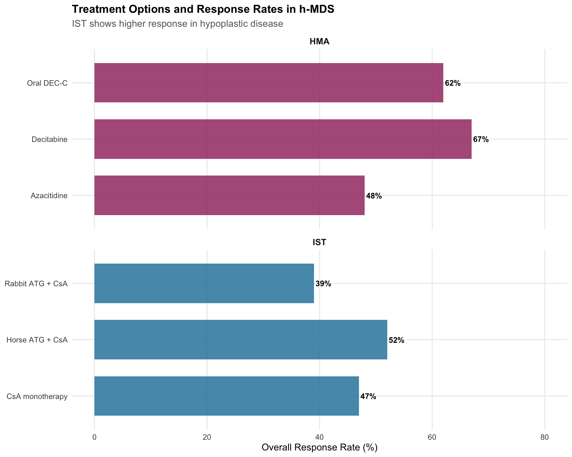
  4, "IST", "Horse ATG + CsA", 52, "First-line",
  4, "IST", "Rabbit ATG + CsA", 39, "Alternative",
  4, "IST", "CsA monotherapy", 47, "If ATG contraindicated",
  5, "HMA", "Azacitidine", 48, "Standard",
  5, "HMA", "Decitabine", 67, "May be superior",
  5, "HMA", "Oral DEC-C", 62, "Equivalent efficacy"
)

ggplot(treatment_flow %>% filter(Step >= 4), 
       aes(x = Option, y = Value, fill = Category)) +
  geom_col(alpha = 0.85, width = 0.7) +
  geom_text(aes(label = paste0(Value, "%")), 
            hjust = -0.1, size = 3.5, fontface = "bold") +
  coord_flip() +
  facet_wrap(~Category, scales = "free_y", ncol = 1) +
  scale_fill_manual(values = c("IST" = "#2E86AB", "HMA" = "#A23B72")) +
  labs(
    x = NULL,
    y = "Overall Response Rate (%)",
    title = "Treatment Options and Response Rates in h-MDS",
    subtitle = "IST shows higher response in hypoplastic disease"
  ) +
  scale_y_continuous(limits = c(0, 80)) +
  theme(
    legend.position = "none",
    strip.text = element_text(face = "bold", size = 11)
  )
Figure 17.1: Treatment algorithm for hypoplastic MDS

17.2 Immunosuppressive Therapy Outcomes

Show code
ist_outcomes <- tribble(
  ~Outcome, ~`ATG + CsA`, ~`CsA Alone`, ~`h-MDS (any IST)`, ~`n-MDS (any IST)`,
  "Overall Response Rate", "49%", "47%", "46-49%", "21-24%",
  "Complete Response", "11%", "8%", "11%", "5%",
  "RBC Transfusion Independence", "30%", "45%", "30-33%", "15%",
  "Median Time to Response", "3-4 months", "2-3 months", "9.4 weeks", "12 weeks",
  "Median Overall Survival", "47 months", "NR", "41.6 months", "35 months",
  "4-year AML Transformation", "—", "—", "14%", "26%"
)

ist_outcomes %>%
  gt() %>%
  tab_header(
    title = "Immunosuppressive Therapy Outcomes",
    subtitle = "h-MDS shows superior response compared to n-MDS"
  ) %>%
  cols_align(align = "center", columns = -Outcome) %>%
  tab_spanner(
    label = "IST Regimen",
    columns = c(`ATG + CsA`, `CsA Alone`)
  ) %>%
  tab_spanner(
    label = "By Cellularity",
    columns = c(`h-MDS (any IST)`, `n-MDS (any IST)`)
  ) %>%
  tab_style(
    style = cell_fill(color = "#E8F5E9"),
    locations = cells_body(columns = `h-MDS (any IST)`)
  ) %>%
  tab_footnote(
    footnote = "NR = Not reached; ATG = Antithymocyte globulin; CsA = Cyclosporine",
    locations = cells_column_labels(columns = Outcome)
  )
Table 17.1
Immunosuppressive Therapy Outcomes
h-MDS shows superior response compared to n-MDS
Outcome1
IST Regimen
By Cellularity
ATG + CsA CsA Alone h-MDS (any IST) n-MDS (any IST)
Overall Response Rate 49% 47% 46-49% 21-24%
Complete Response 11% 8% 11% 5%
RBC Transfusion Independence 30% 45% 30-33% 15%
Median Time to Response 3-4 months 2-3 months 9.4 weeks 12 weeks
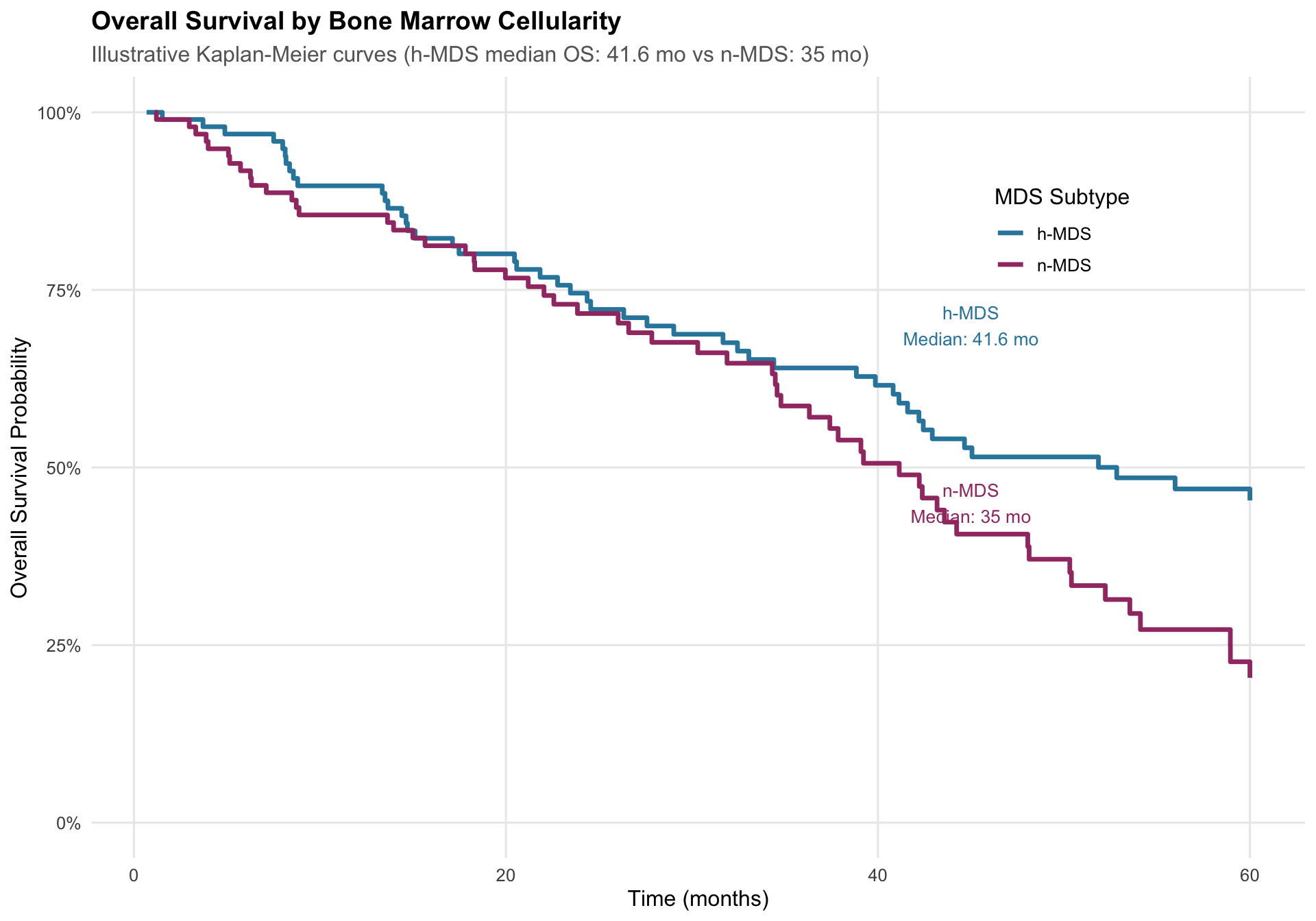
Median Overall Survival 47 months NR 41.6 months 35 months
4-year AML Transformation — — 14% 26%
1 NR = Not reached; ATG = Antithymocyte globulin; CsA = Cyclosporine

17.3 Predictors of IST Response

Show code
ist_predictors <- tribble(
  ~Predictor, ~OR, ~CI_low, ~CI_high, ~p_value,
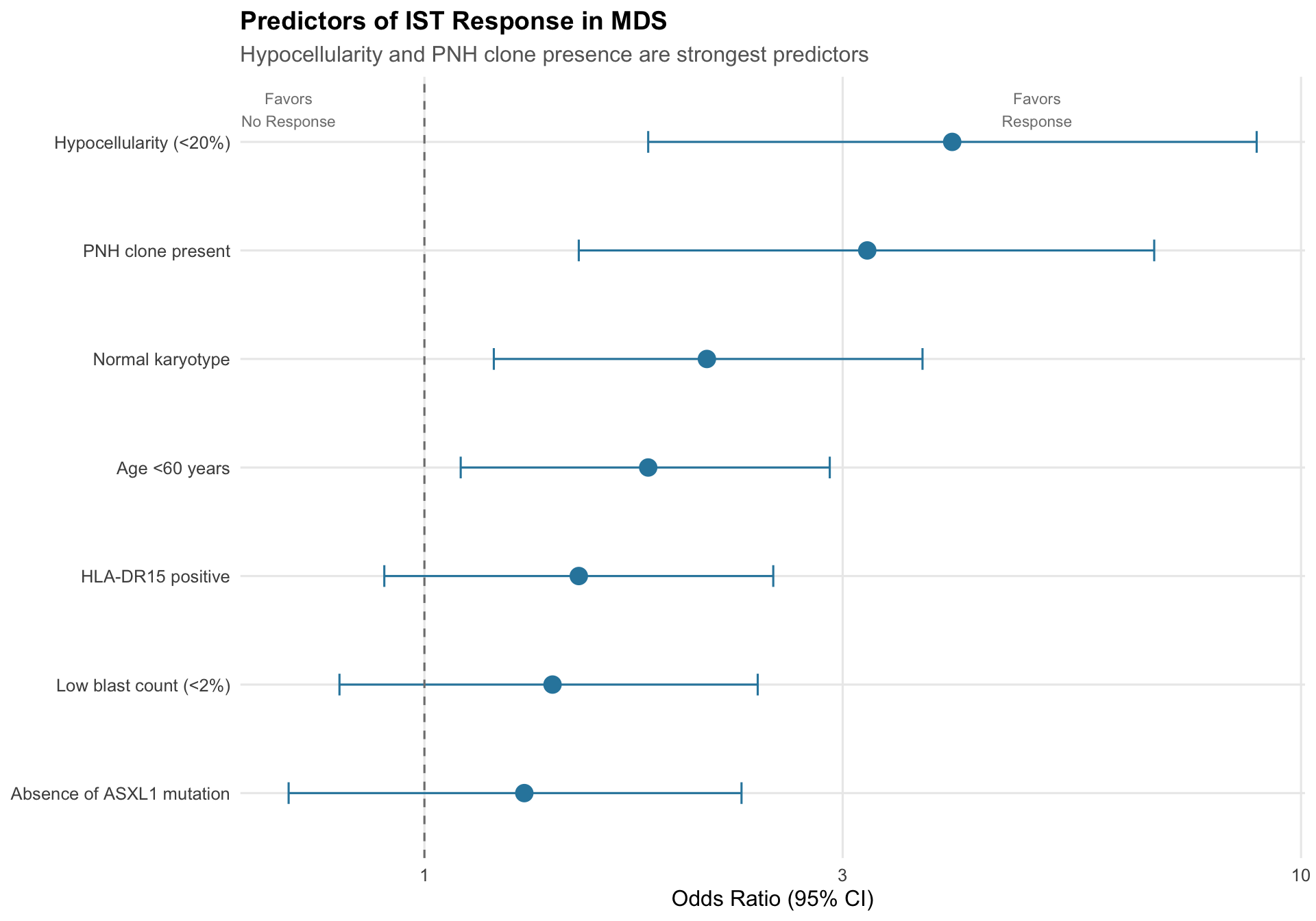
  "Hypocellularity (<20%)", 4.0, 1.8, 8.9, 0.03,
  "PNH clone present", 3.2, 1.5, 6.8, 0.01,
  "Normal karyotype", 2.1, 1.2, 3.7, 0.04,
  "Age <60 years", 1.8, 1.1, 2.9, 0.05,
  "HLA-DR15 positive", 1.5, 0.9, 2.5, 0.12,
  "Low blast count (<2%)", 1.4, 0.8, 2.4, 0.18,
  "Absence of ASXL1 mutation", 1.3, 0.7, 2.3, 0.25
)

ggplot(ist_predictors, aes(x = reorder(Predictor, OR), y = OR)) +
  geom_point(size = 4, color = "#2E86AB") +
  geom_errorbar(aes(ymin = CI_low, ymax = CI_high), width = 0.2, color = "#2E86AB") +
  geom_hline(yintercept = 1, linetype = "dashed", color = "gray50") +
  coord_flip() +
  labs(
    x = NULL,
    y = "Odds Ratio (95% CI)",
    title = "Predictors of IST Response in MDS",
    subtitle = "Hypocellularity and PNH clone presence are strongest predictors"
  ) +
  scale_y_log10() +
  annotate("text", x = 7.3, y = 0.7, label = "Favors\nNo Response", 
           size = 3, color = "gray50") +
  annotate("text", x = 7.3, y = 5, label = "Favors\nResponse", 
           size = 3, color = "gray50")
Figure 17.2: Predictors of response to immunosuppressive therapy in MDS

18 Novel Therapeutic Agents

18.1 Luspatercept

Show code
luspatercept_data <- tribble(
  ~Trial, ~Population, ~`RBC-TI Rate`, ~Comparator, ~`Key Finding`,
  "MEDALIST", "RS+ LR-MDS, ESA-refractory", "38%", "Placebo 13%", "FDA approved 2020",
  "COMMANDS", "RS+ LR-MDS, ESA-naive", "58.5%", "EPO-α 31.2%", "First-line approval 2023",
  "Real-world", "All LR-MDS", "41-48%", "—", "Similar RS+/RS- response"
)

luspatercept_data %>%
  gt() %>%
  tab_header(
    title = "Luspatercept Clinical Trial Results",
    subtitle = "Erythroid maturation agent for lower-risk MDS"
  ) %>%
  cols_align(align = "center", columns = c(`RBC-TI Rate`, Comparator)) %>%
  tab_footnote(
    footnote = "RS = Ring sideroblasts; RBC-TI = Red blood cell transfusion independence",
    locations = cells_column_labels(columns = Population)
  )
Table 18.1
Luspatercept Clinical Trial Results
Erythroid maturation agent for lower-risk MDS
Trial Population1 RBC-TI Rate Comparator Key Finding
MEDALIST RS+ LR-MDS, ESA-refractory 38% Placebo 13% FDA approved 2020
COMMANDS RS+ LR-MDS, ESA-naive 58.5% EPO-α 31.2% First-line approval 2023
Real-world All LR-MDS 41-48% — Similar RS+/RS- response
1 RS = Ring sideroblasts; RBC-TI = Red blood cell transfusion independence

18.2 Imetelstat

Show code
imetelstat_data <- tribble(
  ~Endpoint, ~Imetelstat, ~Placebo, ~`p-value`,
  "8-week RBC-TI", "39.8%", "15.0%", "<0.001",
  "24-week RBC-TI", "28.0%", "3.3%", "<0.001",
  "Median duration of TI", "52 weeks", "13 weeks", "—",
  "VAF reduction (any gene)", "44%", "—", "—",
  "Grade ≥3 neutropenia", "68%", "—", "—"
)

imetelstat_data %>%
  gt() %>%
  tab_header(
    title = "IMerge Trial: Imetelstat in ESA-Refractory LR-MDS",
    subtitle = "FDA approved June 2024"
  ) %>%
  cols_align(align = "center", columns = -Endpoint) %>%
  tab_style(
    style = cell_text(weight = "bold"),
    locations = cells_body(columns = `p-value`, rows = `p-value` == "<0.001")
  ) %>%
  tab_footnote(
    footnote = "VAF = Variant allele frequency; demonstrates disease-modifying activity",
    locations = cells_body(columns = Endpoint, rows = 4)
  )
Table 18.2
IMerge Trial: Imetelstat in ESA-Refractory LR-MDS
FDA approved June 2024
Endpoint Imetelstat Placebo p-value
8-week RBC-TI 39.8% 15.0% <0.001
24-week RBC-TI 28.0% 3.3% <0.001
Median duration of TI 52 weeks 13 weeks —
VAF reduction (any gene)1 44% — —
Grade ≥3 neutropenia 68% — —
1 VAF = Variant allele frequency; demonstrates disease-modifying activity

18.3 TPO-Receptor Agonists

Show code
tpo_data <- tribble(
  ~Agent, ~Setting, ~Response, ~Note,
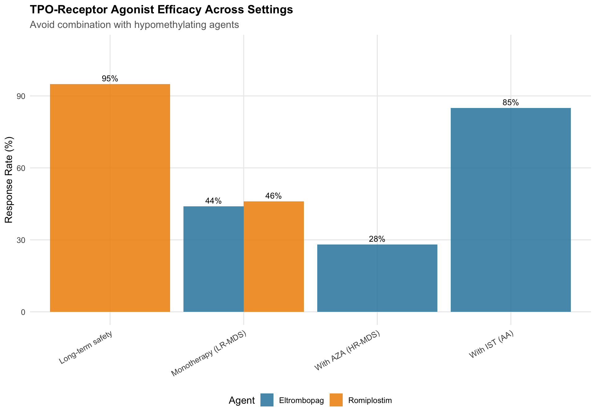
  "Eltrombopag", "Monotherapy (LR-MDS)", 44, "Platelet response",
  "Eltrombopag", "With IST (AA)", 85, "Enhanced response",
  "Eltrombopag", "With AZA (HR-MDS)", 28, "Inferior - avoid",
  "Romiplostim", "Monotherapy (LR-MDS)", 46, "Platelet response",
  "Romiplostim", "Long-term safety", 95, "No excess AML risk"
)

ggplot(tpo_data, aes(x = Setting, y = Response, fill = Agent)) +
  geom_col(position = "dodge", alpha = 0.85) +
  geom_text(aes(label = paste0(Response, "%")), 
            position = position_dodge(width = 0.9),
            vjust = -0.5, size = 3.5) +
  scale_fill_manual(values = c("Eltrombopag" = "#2E86AB", "Romiplostim" = "#F18F01")) +
  labs(
    x = NULL,
    y = "Response Rate (%)",
    fill = "Agent",
    title = "TPO-Receptor Agonist Efficacy Across Settings",
    subtitle = "Avoid combination with hypomethylating agents"
  ) +
  theme(axis.text.x = element_text(angle = 30, hjust = 1)) +
  scale_y_continuous(limits = c(0, 110))
Figure 18.1: TPO-receptor agonist efficacy in MDS with thrombocytopenia

19 Transplant Outcomes

19.1 Allogeneic HSCT Results in h-MDS

Show code
transplant_data <- tribble(
  ~Outcome, ~`h-MDS`, ~`n-MDS`, ~`Comments`,
  "Overall Survival (3-year)", "72.7%", "50-55%", "Favorable in hypoplastic",
  "Relapse-Free Survival", "72.7%", "45-50%", "Lower relapse rate",
  "Relapse Rate", "0-10%", "25-35%", "Significantly lower",
  "NRM (2-year)", "15-20%", "20-25%", "Similar",
  "Myeloid Engraftment (median)", "Day 11", "Day 14", "Faster engraftment",
  "Platelet Engraftment (median)", "Day 10", "Day 15", "Faster engraftment"
)

transplant_data %>%
  gt() %>%
  tab_header(
    title = "Allogeneic HSCT Outcomes by Bone Marrow Cellularity",
    subtitle = "h-MDS patients show favorable transplant outcomes"
  ) %>%
  cols_align(align = "center", columns = c(`h-MDS`, `n-MDS`)) %>%
  tab_style(
    style = cell_fill(color = "#E8F5E9"),
    locations = cells_body(columns = `h-MDS`)
  ) %>%
  tab_footnote(
    footnote = "NRM = Non-relapse mortality",
    locations = cells_body(columns = Outcome, rows = 4)
  )
Table 19.1
Allogeneic HSCT Outcomes by Bone Marrow Cellularity
h-MDS patients show favorable transplant outcomes
Outcome h-MDS n-MDS Comments
Overall Survival (3-year) 72.7% 50-55% Favorable in hypoplastic
Relapse-Free Survival 72.7% 45-50% Lower relapse rate
Relapse Rate 0-10% 25-35% Significantly lower
NRM (2-year)1 15-20% 20-25% Similar
Myeloid Engraftment (median) Day 11 Day 14 Faster engraftment
Platelet Engraftment (median) Day 10 Day 15 Faster engraftment
1 NRM = Non-relapse mortality

19.2 Adverse Prognostic Factors for Transplant

Show code
adverse_factors <- tribble(
  ~Factor, ~`Impact on Outcome`, ~`HR/OR`, ~`Recommendation`,
  "TP53 multihit", "Very poor OS and RFS", "HR 2.5-4.0", "Consider clinical trial",
  "ASXL1 mutation", "Inferior OS", "HR 1.5-2.0", "Proceed if eligible",
  "RUNX1 mutation", "Higher relapse", "HR 1.4-1.8", "Consider intensification",
  "Complex karyotype", "Poor outcomes", "HR 2.0-3.0", "Early transplant",
  "High transfusion burden", "Higher NRM", "OR 1.8", "Iron chelation pre-HCT",
  "MRD positive pre-HCT", "Higher relapse", "HR 2.5", "Consider bridging therapy"
)

adverse_factors %>%
  gt() %>%
  tab_header(
    title = "Adverse Prognostic Factors for HSCT in h-MDS"
  ) %>%
  cols_align(align = "center", columns = c(`HR/OR`)) %>%
  tab_style(
    style = cell_fill(color = "#FFEBEE"),
    locations = cells_body(rows = Factor == "TP53 multihit")
  )
Table 19.2
Adverse Prognostic Factors for HSCT in h-MDS
Factor Impact on Outcome HR/OR Recommendation
TP53 multihit Very poor OS and RFS HR 2.5-4.0 Consider clinical trial
ASXL1 mutation Inferior OS HR 1.5-2.0 Proceed if eligible
RUNX1 mutation Higher relapse HR 1.4-1.8 Consider intensification
Complex karyotype Poor outcomes HR 2.0-3.0 Early transplant
High transfusion burden Higher NRM OR 1.8 Iron chelation pre-HCT
MRD positive pre-HCT Higher relapse HR 2.5 Consider bridging therapy

20 Prognosis and Risk Stratification

20.1 IPSS-R Distribution in h-MDS

Show code
ipss_data <- tribble(
  ~Risk_Category, ~h_MDS, ~n_MDS,
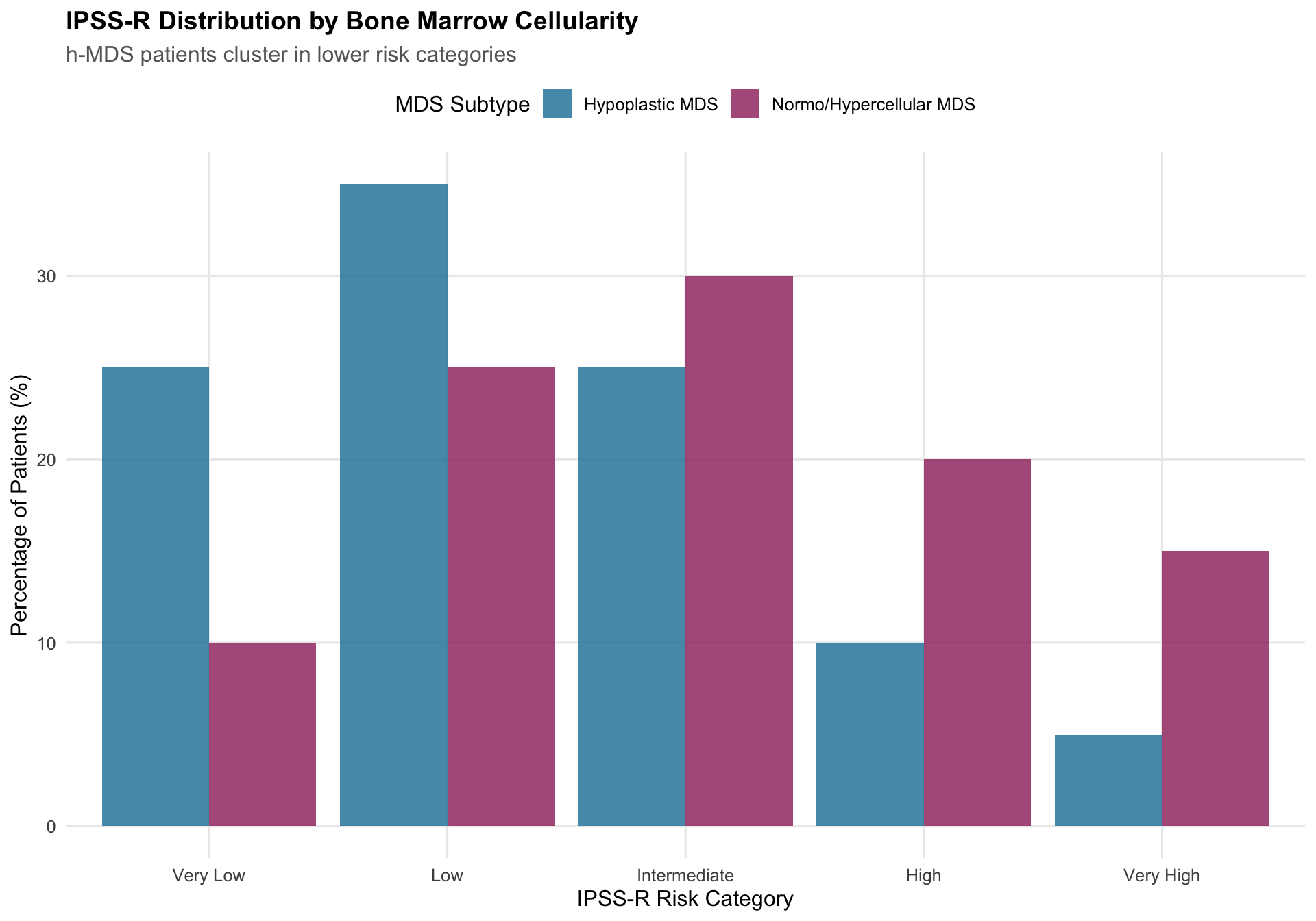
  "Very Low", 25, 10,
  "Low", 35, 25,
  "Intermediate", 25, 30,
  "High", 10, 20,
  "Very High", 5, 15
) %>%
  mutate(Risk_Category = factor(Risk_Category, 
                                 levels = c("Very Low", "Low", "Intermediate", 
                                           "High", "Very High")))

ipss_long <- ipss_data %>%
  pivot_longer(cols = c(h_MDS, n_MDS),
               names_to = "Type",
               values_to = "Percentage") %>%
  mutate(Type = ifelse(Type == "h_MDS", "Hypoplastic MDS", "Normo/Hypercellular MDS"))

ggplot(ipss_long, aes(x = Risk_Category, y = Percentage, fill = Type)) +
  geom_col(position = "dodge", alpha = 0.85) +
  scale_fill_manual(values = c("Hypoplastic MDS" = "#2E86AB",
                               "Normo/Hypercellular MDS" = "#A23B72")) +
  labs(
    x = "IPSS-R Risk Category",
    y = "Percentage of Patients (%)",
    fill = "MDS Subtype",
    title = "IPSS-R Distribution by Bone Marrow Cellularity",
    subtitle = "h-MDS patients cluster in lower risk categories"
  ) +
  theme(legend.position = "top")
Figure 20.1: IPSS-R risk category distribution by MDS cellularity

20.2 Survival Outcomes

Show code
# Simulated survival data for illustration
set.seed(123)
n_patients <- 200

survival_data <- tibble(
  patient_id = 1:n_patients,
  subtype = rep(c("h-MDS", "n-MDS"), each = n_patients/2),
  time = c(
    rweibull(n_patients/2, shape = 1.2, scale = 50),  # h-MDS
    rweibull(n_patients/2, shape = 1.2, scale = 38)   # n-MDS
  ),
  status = rbinom(n_patients, 1, 0.6)
) %>%
  mutate(time = pmin(time, 60))  # Cap at 60 months

# Calculate KM-like survival probabilities
km_data <- survival_data %>%
  group_by(subtype) %>%
  arrange(time) %>%
  mutate(
    n_at_risk = n():1,
    surv_prob = cumprod(1 - status/n_at_risk)
  ) %>%
  distinct(time, .keep_all = TRUE)

ggplot(km_data, aes(x = time, y = surv_prob, color = subtype)) +
  geom_step(linewidth = 1.2) +
  scale_color_manual(values = c("h-MDS" = "#2E86AB", "n-MDS" = "#A23B72")) +
  scale_y_continuous(labels = scales::percent, limits = c(0, 1)) +
  labs(
    x = "Time (months)",
    y = "Overall Survival Probability",
    color = "MDS Subtype",
    title = "Overall Survival by Bone Marrow Cellularity",
    subtitle = "Illustrative Kaplan-Meier curves (h-MDS median OS: 41.6 mo vs n-MDS: 35 mo)"
  ) +
  theme(legend.position = c(0.8, 0.8)) +
  annotate("text", x = 45, y = 0.7, label = "h-MDS\nMedian: 41.6 mo", 
           color = "#2E86AB", size = 3.5) +
  annotate("text", x = 45, y = 0.45, label = "n-MDS\nMedian: 35 mo", 
           color = "#A23B72", size = 3.5)
Figure 20.2: Overall survival comparison by MDS subtype (illustrative)

21 Summary and Conclusions

21.1 Key Practice Points

Show code
practice_points <- tribble(
  ~Domain, ~Recommendation,
  "Diagnosis", "Apply WHO 2022 criteria: cellularity <30% (<70y) or <20% (≥70y) with dysplasia",
  "Workup", "Include NGS panel, cytogenetics, PNH clone assessment, and hg-score calculation",
  "Risk stratification", "Use both IPSS-R and IPSS-M; most h-MDS patients are lower risk",
  "AA-like phenotype", "PNH+, low hg-score → Consider IST with horse ATG + cyclosporine first",
  "MDS-like phenotype", "High-risk genetics → HMA-based therapy; consider VEN combination",
  "IST response prediction", "Hypocellularity <20%, PNH clone, normal karyotype predict response",
  "Novel agents", "Luspatercept (anemia), Imetelstat (ESA-refractory), Eltrombopag (thrombocytopenia)",
  "Transplant", "Favorable outcomes; consider early if high-risk features; avoid with TP53 multihit",
  "Monitoring", "Regular CBC, marrow reassessment if disease evolution suspected"
)

practice_points %>%
  gt() %>%
  tab_header(
    title = "Clinical Practice Points for Hypoplastic MDS"
  ) %>%
  cols_width(
    Domain ~ px(150),
    Recommendation ~ px(500)
  ) %>%
  tab_style(
    style = cell_text(weight = "bold"),
    locations = cells_body(columns = Domain)
  ) %>%
  tab_style(
    style = cell_fill(color = "#E3F2FD"),
    locations = cells_body(rows = Domain %in% c("AA-like phenotype", "IST response prediction"))
  )
Table 21.1
Clinical Practice Points for Hypoplastic MDS
Domain Recommendation
Diagnosis Apply WHO 2022 criteria: cellularity <30% (<70y) or <20% (≥70y) with dysplasia
Workup Include NGS panel, cytogenetics, PNH clone assessment, and hg-score calculation
Risk stratification Use both IPSS-R and IPSS-M; most h-MDS patients are lower risk
AA-like phenotype PNH+, low hg-score → Consider IST with horse ATG + cyclosporine first
MDS-like phenotype High-risk genetics → HMA-based therapy; consider VEN combination
IST response prediction Hypocellularity <20%, PNH clone, normal karyotype predict response
Novel agents Luspatercept (anemia), Imetelstat (ESA-refractory), Eltrombopag (thrombocytopenia)
Transplant Favorable outcomes; consider early if high-risk features; avoid with TP53 multihit
Monitoring Regular CBC, marrow reassessment if disease evolution suspected

21.2 Research Directions

Future investigations in hypoplastic MDS should focus on:

  1. Biomarker development for predicting IST vs HMA response
  2. Combination strategies integrating IST with novel agents
  3. MRD assessment using NGS-based approaches
  4. Germline predisposition screening in younger patients
  5. Novel immune-modulating agents targeting specific T-cell populations

22 Session Information

Show code
sessionInfo()
R version 4.6.1 (2026-06-24)
Platform: aarch64-apple-darwin23
Running under: macOS Tahoe 26.6

Matrix products: default
BLAS:   /Library/Frameworks/R.framework/Versions/4.6/Resources/lib/libRblas.0.dylib 
LAPACK: /Library/Frameworks/R.framework/Versions/4.6/Resources/lib/libRlapack.dylib;  LAPACK version 3.12.1

locale:
[1] en_US.UTF-8/en_US.UTF-8/en_US.UTF-8/C/en_US.UTF-8/en_US.UTF-8

time zone: America/Chicago
tzcode source: internal

attached base packages:
[1] stats     graphics  grDevices utils     datasets  methods   base     

other attached packages:
 [1] viridis_0.6.5     viridisLite_0.4.3 scales_1.4.0      kableExtra_1.4.1 
 [5] gt_1.3.0          lubridate_1.9.5   forcats_1.0.1     stringr_1.6.0    
 [9] dplyr_1.2.1       purrr_1.2.2       readr_2.2.0       tidyr_1.3.2      
[13] tibble_3.3.1      ggplot2_4.0.3     tidyverse_2.0.0  

loaded via a namespace (and not attached):
 [1] sass_0.4.10        generics_0.1.4     xml2_1.6.0         stringi_1.8.7     
 [5] hms_1.1.4          digest_0.6.39      magrittr_2.0.5     evaluate_1.0.5    
 [9] grid_4.6.1         timechange_0.4.0   RColorBrewer_1.1-3 fastmap_1.2.0     
[13] jsonlite_2.0.0     gridExtra_2.3.1    textshaping_1.0.5  cli_3.6.6         
[17] rlang_1.3.0        withr_3.0.3        yaml_2.3.12        otel_0.2.0        
[21] tools_4.6.1        tzdb_0.5.0         vctrs_0.7.3        R6_2.6.1          
[25] lifecycle_1.0.5    fs_2.1.0           htmlwidgets_1.6.4  pkgconfig_2.0.3   
[29] pillar_1.11.1      gtable_0.3.6       glue_1.8.1         systemfonts_1.3.2 
[33] xfun_0.60          tidyselect_1.2.1   rstudioapi_0.19.0  knitr_1.51        
[37] farver_2.1.2       htmltools_0.5.9    labeling_0.4.3     rmarkdown_2.31    
[41] svglite_2.2.2      compiler_4.6.1     S7_0.2.2          

References

Garcia, Jacqueline S., Uwe Platzbecker, Olatoyosi Odenike, et al. 2025. “Efficacy and Safety of Venetoclax Plus Azacitidine for Patients with Treatment-Naive High-Risk Myelodysplastic Syndromes.” Blood 145 (11): 1126–35. https://doi.org/10.1182/blood.2024025464.
Hong, Lih En, Mihir D. Wechalekar, Monika Kutyna, et al. 2024. “IDH-Mutant Myeloid Neoplasms Are Associated with Seronegative Rheumatoid Arthritis and Innate Immune Activation.” Blood 143 (18): 1873–77. https://doi.org/10.1182/blood.2023023593.
Komrokji, Rami S., Luis E. Aguirre, Najla H. Al Ali, et al. 2023. “Activity of Luspatercept and ESAs Combination for Treatment of Anemia in Lower-Risk Myelodysplastic Syndromes.” Blood Advances 7 (14): 3677–79. https://doi.org/10.1182/bloodadvances.2023009781.
Raddi, Marco Gabriele, Sophie Park, Michaela Fontenay, et al. 2025. “IPSS-m Risk and Specific Sex-Associated Somatic Mutations Predict Response to ESA Therapy in LR-MDS: Building a New Score.” Blood Journal, ahead of print, June 25. https://doi.org/10.1182/blood.2024027540.
Sasaki, Koji, Elias Jabbour, Guillermo Montalban-Bravo, et al. 2022. “Low-Dose Decitabine Versus Low-Dose Azacitidine in Lower-Risk MDS.” NEJM Evidence 1 (10). https://doi.org/10.1056/EVIDoa2200034.
Sekeres, Mikkael, Ahmed Hnoosh, Aylin Yucel, et al. 2025. “Real-World Treatment Patterns and Outcomes of First-Line Luspatercept in Patients with Myelodysplastic Syndromes in the United States.” Blood 146 (Supplement 1): 5638–38. https://doi.org/10.1182/blood-2025-5638.
Urrutia, Samuel, Koji Sasaki, Alex Bataller, et al. 2024. “Oral Decitabine/Cedazuridine in Patients with MDS and TP53 Mutations: A Propensity Score Matching Analysis from the Phase II and III Trials.” Blood 144 (Supplement 1): 661–61. https://doi.org/10.1182/blood-2024-193274.
Vu, Binh T., Romyr Dominique, Bruce J. Fahr, et al. 2024. “Discovery of Rezatapopt (PC14586), a First-in-Class, Small-Molecule Reactivator of P53 Y220C Mutant in Development.” ACS Medicinal Chemistry Letters 16 (1): 34–39. https://doi.org/10.1021/acsmedchemlett.4c00379.
Zampini, Matteo, Elena Riva, Luca Lanino, et al. 2025. “Characterization and Clinical Implications of P53 Dysfunction in Patients with Myelodysplastic Syndromes.” Journal of Clinical Oncology, ahead of print, May 2. https://doi.org/10.1200/jco-24-02394.
Zeidan, Amer M., Uwe Platzbecker, Jan Philipp Bewersdorf, et al. 2023. “Consensus Proposal for Revised International Working Group Response Criteria for Higher Risk Myelodysplastic Syndromes.” Blood, ahead of print, February 1. https://doi.org/10.1182/blood.2022018604.